![]()
AWK can be used in a non GUI environment as a pretty impressive, if limited Spreadsheet simulation to generate the correct data at each stage of a basic stats process that you may do in a tech maths class for example. It is limited by it's in built maths functions, which are still considerable:
- Calling Built-in: How to call built-in functions.
- Numeric Functions: Functions that work with numbers, including
int,sinandrand. - String Functions: Functions for string manipulation, such as
split,match, andsprintf. - I/O Functions: Functions for files and shell commands.
- Time Functions: Functions for dealing with time stamps.
https://www.math.utah.edu/docs/info/gawk_13.html#SEC125
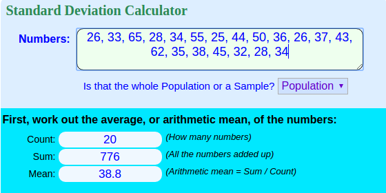
In statistics, the first stages usually involve finding the mean or average value of a data set, which is the sum of the samples divided by the total.
Using a simple data set of 20 "travel times": cat traveltimes.txt
26, 33, 65, 28, 34, 55, 25, 44, 50, 36, 26, 37, 43, 62, 35, 38, 45, 32, 28, 34
from https://www.mathsisfun.com/data/standard-normal-distribution.html
and checking the results here:
https://www.mathsisfun.com/data/standard-deviation-calculator.html
First, set up the BEGIN, pre loop section with the correct delimiter to separate the CSV fields into records and show the sample list above in the file traveltimes.txt as a column:
awk 'BEGIN{RS=", " } {ORS="\n"; print $1}' traveltimes.txt
26
33
65
28
34
55
25
44
50
36
26
37
43
62
35
38
45
32
28
34
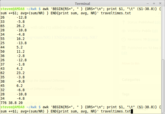
Now a sum total can be generated of the sample values in column $1 and as the NR (No. of Records) is counted by default by awk, it can be used to divide the total and provide an average and a count:
awk 'BEGIN{RS=", " } {ORS="\n"; print $1} {sum +=$1; avg=(sum/NR)} END{print sum, avg, NR}' traveltimes.txt
26
33
65
28
34
55
25
44
50
36
26
37
43
62
35
38
45
32
28
34
776 38.8 20
These correlate with the webpage calculator above:

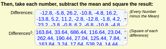
The mean (avg) is 38.8, so subtract this from $1 and print it for each record, with tabs (\t) added to tidy the columns:
awk 'BEGIN{RS=", " } {ORS="\n"; print $1, "\t" ($1-38.8)} {sum +=$1; avg=(sum/NR) } END{print sum, avg, NR}' traveltimes.txt
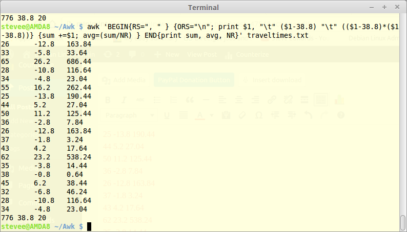
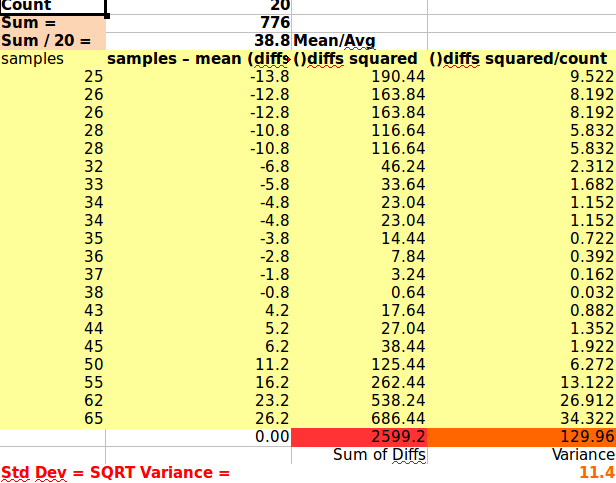
Now calculate the Variance:

This means first square all those column 2 differences, with tabs for clarity while at it:
awk 'BEGIN{RS=", " } {ORS="\n"; print $1, "\t" ($1-38.8) "\t" (($1-38.8)*($1-38.8))} {sum +=$1; avg=(sum/NR) } END{print sum, avg, NR}' traveltimes.txt
These columns can now have variables assigned to their calculations in the main loop body, and summed in the END section also using the variable names as print references. The seemingly nonsense exponential is small scale rounding for zero!:
awk 'BEGIN{RS=", " } {ORS="\n"; print $1, "\t\t" ($1-38.8) "\t\t" (($1-38.8)*($1-38.8))} {sum +=$1; avg=(sum/NR); sum2+=($1-38.8); sum3+=(($1-38.8)*($1-38.8)) } END{print sum, avg, NR, "\t" sum2, "\t" sum3}' traveltimes.txt
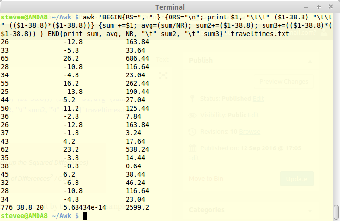
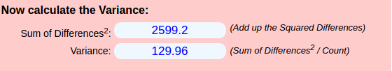
The Variance can be calculated from the differences squared sum (2599.2) by dividing it by the number of samples (20), which needs to be evaluated again as NR for use as the divisor (20) in the END section:
awk 'BEGIN{RS=", " } {ORS="\n"; print $1, "\t\t" ($1-38.8) "\t\t" (($1-38.8)*($1-38.8))} {sum +=$1; avg=(sum/NR); sum2+=($1-38.8); sum3+=(($1-38.8)*($1-38.8)) } END{print sum, avg, NR, "\t" sum2, "\t" sum3, sum3/20}' traveltimes.txt
776 38.8 20 5.68434e-14 2599.2 129.96
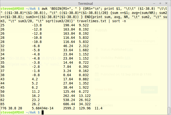
The Std Dev is found by adding yet another calculation to the END print arguments:
awk 'BEGIN{RS=", " } {ORS="\n"; print $1, "\t\t" ($1-38.8) "\t\t" (($1-38.8)*($1-38.8))} {sum +=$1; avg=(sum/NR); sum2+=($1-38.8); sum3+=(($1-38.8)*($1-38.8)) } END{print sum, avg, NR, "\t" sum2, "\t" sum3, sum3/20, sqrt(sum3/20)}' traveltimes.txt
776 38.8 20 5.68434e-14 2599.2 129.96 11.4

For all final sorted columns as per Libre comparison below - the decimal exponent should be rounded to 1 significant figure in awk to get 0 also but needs printf %d which complicates it; as I had to do in Libre - but the small exponent value was the same as Awk showed:
awk 'BEGIN{RS=", " } {ORS="\n"; print $1, "\t\t" ($1-38.8) "\t\t" (($1-38.8)*($1-38.8)), "\t" (($1-38.8)*($1-38.8))/20} {sum +=$1; avg=(sum/NR); sum2+=($1-38.8); sum3+=(($1-38.8)*($1-38.8)) } END{print sum, avg, NR, "\t" sum2, "\t" sum3, "\t" sum3/20, "\t" sqrt(sum3/20)}' traveltimes.txt | sort -n
Awk is pretty impressive as a text based spreadsheet imitator eh?!
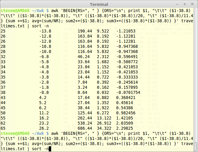
If you want to know how many StdDevs away from the Mean each value is, remove the END section and divide $2 by the StdDev (11.4) to give the "Z" score:
awk 'BEGIN{RS=", " } {ORS="\n"; print $1, "\t\t" ($1-38.8) "\t\t" (($1-38.8)*($1-38.8)), "\t" (($1-38.8)*($1-38.8))/20, "\t" ($1-38.8)/11.4} {sum +=$1; avg=(sum/NR); sum2+=($1-38.8); sum3+=(($1-38.8)*($1-38.8)) }' traveltimes.txt | sort -n
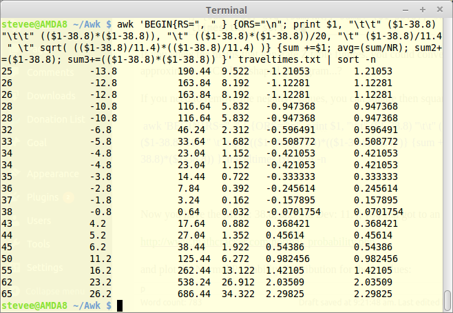
If you need to remove the negative values, you can square then square root the values and add a space before the tab:
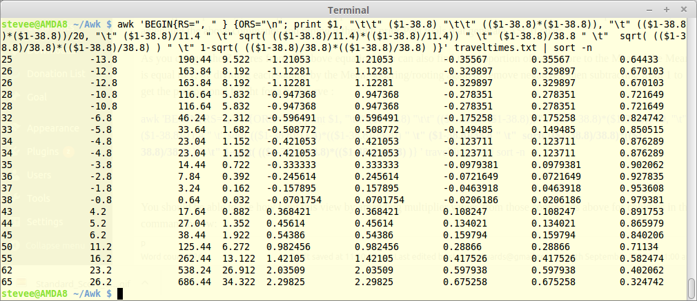
awk 'BEGIN{RS=", " } {ORS="\n"; print $1, "\t\t" ($1-38.8) "\t\t" (($1-38.8)*($1-38.8)), "\t" (($1-38.8)*($1-38.8))/20, "\t" ($1-38.8)/11.4 " \t" sqrt( (($1-38.8)/11.4)*(($1-38.8)/11.4) )} {sum +=$1; avg=(sum/NR); sum2+=($1-38.8); sum3+=(($1-38.8)*($1-38.8)) }' traveltimes.txt | sort -n
Although not precise, you can generate an approximate ASCII bell curve of the Std Normal Distribution probabilities by amending the above commands and piping it through prior Post tools that generate ASCII chars.
As you can get the Z scores from the above equation, you can also find the proportion of each score to the Mean if the Mean is equal to 1, by dividing each sample by the Mean, squaring/rooting again to remove negatives, then subtracting from 1 to get the proportional height of the probabilities for a rough bell curve :
awk 'BEGIN{RS=", " } {ORS="\n"; print $1, "\t\t" ($1-38.8) "\t\t" (($1-38.8)*($1-38.8)), "\t" (($1-38.8)*($1-38.8))/20, "\t" ($1-38.8)/11.4 " \t" sqrt( (($1-38.8)/11.4)*(($1-38.8)/11.4)) " \t" ($1-38.8)/38.8 " \t" sqrt( (($1-38.8)/38.8)*(($1-38.8)/38.8) ) " \t" 1-sqrt( (($1-38.8)/38.8)*(($1-38.8)/38.8) )} ' traveltimes.txt | sort -n
You should be able to see how I got this "bell" view by amending multiplier values from those commands above for columns in the command below and piping it though the ASCII generator after multiplying the final column values by 100%:
awk 'BEGIN{RS=", " } {ORS="\n"; print $1, "\t\t" ($1-38.8) "\t\t" (($1-38.8)*($1-38.8)), "\t" (($1-38.8)*($1-38.8))/20, "\t" ($1-38.8)/11.4 " \t" sqrt( (($1-38.8)/11.4)*(($1-38.8)/11.4)) " \t" ($1-38.8)/38.8 " \t" sqrt( (($1-38.8)/38.8)*(($1-38.8)/38.8) ) " \t" 1-sqrt( (($1-38.8)/38.8)*(($1-38.8)/38.8) ) " \t" 100*(1-sqrt( (($1-38.8)/38.8)*(($1-38.8)/38.8))) }' traveltimes.txt | sort -n | awk '{print $1,$9}' | awk '{print $1,$2}' | awk '!max{max=$2;}{r="";i=s=50*$2/max;while(i-->0)r=r"#";printf "%15s %5d %s %s",$2,$1,r,"\n";}'
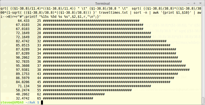
As duplicates don't show in a bell curve, they can be removed with uniq after sort:
awk 'BEGIN{RS=", " } {ORS="\n"; print $1, "\t\t" ($1-38.8) "\t\t" (($1-38.8)*($1-38.8)), "\t" (($1-38.8)*($1-38.8))/20, "\t" ($1-38.8)/11.4 " \t" sqrt( (($1-38.8)/11.4)*(($1-38.8)/11.4)) " \t" ($1-38.8)/38.8 " \t" sqrt( (($1-38.8)/38.8)*(($1-38.8)/38.8) ) " \t" 1-sqrt( (($1-38.8)/38.8)*(($1-38.8)/38.8) ) " \t" 100*(1-sqrt( (($1-38.8)/38.8)*(($1-38.8)/38.8))) }' traveltimes.txt | sort -n | uniq | awk '{print $1,$9}' | awk '{print $1,$2}' | awk '!max{max=$2;}{r="";i=s=50*$2/max;while(i-->0)r=r"#";printf "%15s %5d %s %s",$2,$1,r,"\n";}'
This may be useful to you in linux because I could not - for the life of me - find how to generate a Normal Dist curve in Libre Calc or Gnumeric! Hence the webpage example below.
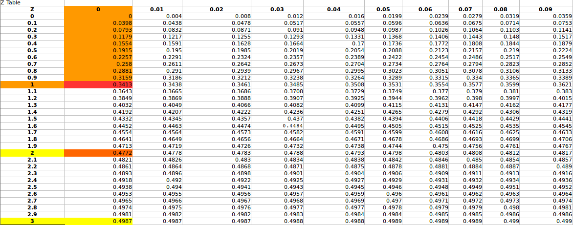
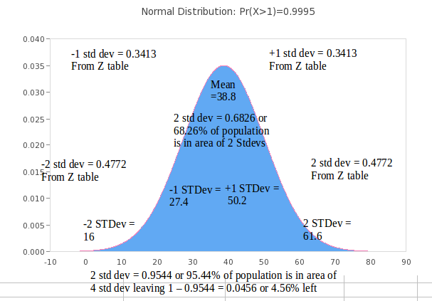
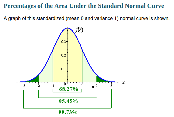
Just bear in mind these proportions may not be quite the same as the Z table values below, as they relate the Std Dev to the total area under a Normal Distribution, but close enough for ASCII values:
https://statistics.laerd.com/statistical-guides/standard-score.php
https://en.wikipedia.org/wiki/Standard_normal_table
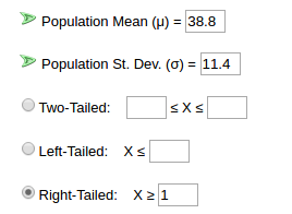
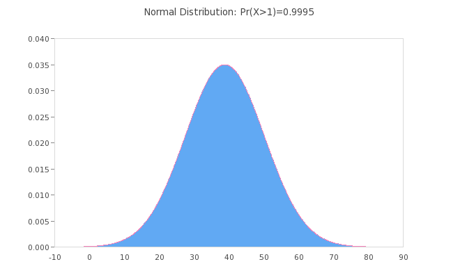
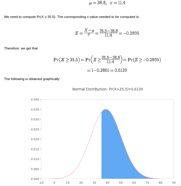
As you have the Mean: 38.8; and Std Dev: 11.4, you can go to an online grapher site like:
https://www.mathcracker.com/normal_probability.php
and plot the Normal Probability Distribution for these values:
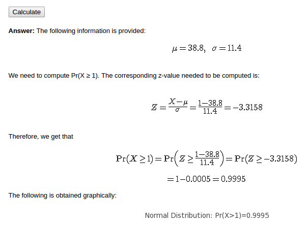
cat traveltimes.txt
26, 33, 65, 28, 34, 55, 25, 44, 50, 36, 26, 37, 43, 62, 35, 38, 45, 32, 28, 34
However, you need to understand that these example figures do NOT follow a Normal Distribution, which requires symmetry as above, because they have asymmetrical Std Devs (11.4) from the Mean of 38.8; about 2 Std Devs up to 65 max to the right of centre from the Mean, and just over 1 Std down to 25 to the left. This Post is to show Awk's abilities, not explain Statistics, however it's interesting:
https://statistics.laerd.com/statistical-guides/standard-score.php
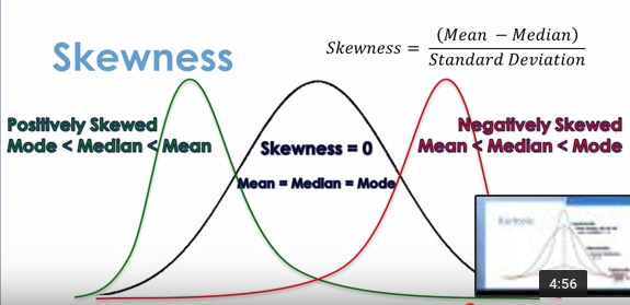
The above samples are positively skewed as the mean (38.8) is greater than the median (35.5), as there is more data to the right of the mean, up to 65.
If the median (35.5) is included for a right tailed set it gives:
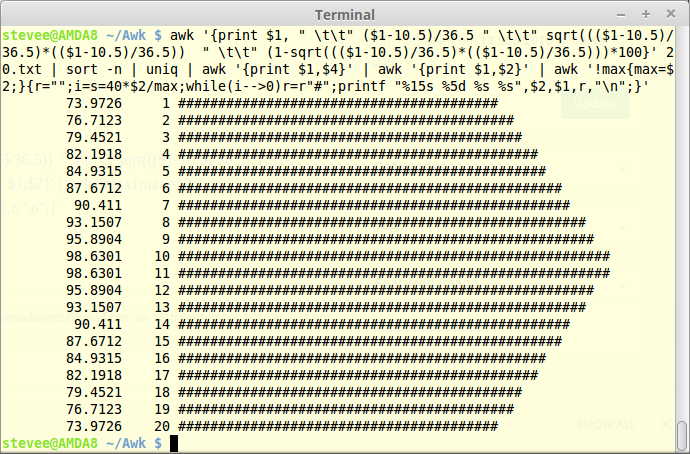
Here's another example you can check for the numbers:
cat 20.txt
1.00
2.00
3.00
4.00
5.00
6.00
7.00
8.00
9.00
10.00
11.00
12.00
13.00
14.00
15.00
16.00
17.00
18.00
19.00
20.00
20.00
19.00
18.00
17.00
16.00
15.00
14.00
13.00
12.00
11.00
10.00
9.00
8.00
7.00
6.00
5.00
4.00
3.00
2.00
1.00
awk '{print $1, " \t\t" ($1-10.5)/36.5 " \t\t" sqrt((($1-10.5)/36.5)*(($1-10.5)/36.5)) " \t\t" (1-sqrt((($1-10.5)/36.5)*(($1-10.5)/36.5)))*100}' 20.txt | sort -n | uniq | awk '{print $1,$4}' | awk '{print $1,$2}' | awk '!max{max=$2;}{r="";i=s=40*$2/max;while(i-->0)r=r"#";printf "%15s %5d %s %s",$2,$1,r,"\n";}'